Excel, a versatile tool for organization and data management, is featured with a myriad of functions and one of them is freezing rows. This article will guide you on how to freeze top two rows in Excel, ensuring that no matter how far you navigate down, the top two rows remain visible. The key points of our discussion will revolve around three main facets - understanding the basics of freezing rows in Excel, taking a step-by-step journey on how you can freeze the top two rows, and illuminating how to customise and manage frozen rows in Excel. So whether you're a professional seeking to intensify your Excel proficiency, or a novice trying to find your way around it, this article is for you. Let's dive right in, starting with understanding the basics of freezing rows in Excel. These foundations lay the bedrock for our discussion, setting off on a promising note.

Understanding the Basics of Freezing Rows in Excel

Excel, a powerful tool packed with numerous features that simplify data manipulation, offers the capability to freeze rows and columns, enhancing visibility and ease of navigation. But what does freezing rows entail, and why is it necessary? This intricate guide aims to equip readers with a comprehensive understanding on the basics of freezing rows in Excel, carefully dissecting the rationale behind freezing rows, the various types of freeze panes available, and the prerequisites for this operation. Firstly, we'll explore the reasons for freezing rows in Excel; these could stem from maintaining header visibility to seamlessly navigating through vast datasets. Next, we'll delve into the different types of freeze panes compatible with unique datasets, serving diverse needs. Lastly, we'll venture into the prerequisites needed for the freezing of rows. Understanding these fundamental aspects lays the groundwork towards mastering the art of freezing rows in Excel. In the upcoming section, we'll delve deeper into why we need to freeze rows, setting the stage for our exploration. It's time to turn these digital ice ages into periods of productivity and efficiency. Get ready to delve deep into the sea of Excel rows, the next time won’t leave you freezing in panic but instead keep you afloat with confidence.

Why Freeze Rows in Excel?

Understanding the basics of freezing rows in Excel is crucial for anyone handling voluminous data on a regular day-to-day basis. Freezing rows in Excel, also known as 'locking' rows, is a very helpful feature that streamlines data analysis and manipulation in an Excel worksheet. When you're working with large datasets, information can stretch beyond your screen's view, and you may need to scroll down to view more rows. This action would typically cause the top rows to disappear from view, making it difficult to remember what each column represents. That's where freezing rows come into play. Excel's freeze rows feature allows you to keep specific rows or columns visible while you're scrolling through the rest of your worksheet. This is particularly valuable when your sheet has several columns of key data that serve as reference points for the rest. By freezing these rows, you can scroll down to view more data while keeping your headings in sight. This feature enhances accuracy and efficiency by preventing confusion from losing sight of column headers. Additionally, freezing rows in Excel comes in handy during data comparisons. It's not uncommon to need to compare values from different sections of an Excel spreadsheet. If these sections are distant apart, navigating between them can be inconvenient. By freezing rows, you can keep one section in view while scrolling to another, making it significantly easier and faster to compare data. In collaborative settings, freezing rows can also promote clarity and coherence. If the worksheet gets shared among several people, frozen rows serve as a static reference point that everyone can see. This helps ensure that everyone is literally on the same page in terms of what information they are viewing and referencing. Using the freeze rows function in Excel can also help with data presentation. The static view of headers and other important information makes your spreadsheet easier to read, understand, and interpret. It gives your spreadsheet a well-structured look, which not only helps with data manipulation and interpretation, but also adds a level of professionalism to your work. In summary, freezing rows in Excel is a feature designed to save time, increase accuracy, enhance data analysis, facilitate collaboration, and ultimately, to improve productivity. Whether for personal or professional use, understanding how to freeze rows in Excel is a vital skill for efficient data handling and management. The benefits are multifold and the feature easy to use, making it a must-know for anyone who uses Excel regularly.

Types of Freeze Panes in Excel

Excel is a powerful tool that offers a plethora of features to handle and manipulate data efficiently. One of these features is the 'Freeze Panes,' which is a lifesaver for handling large datasets. Under the 'Freeze Panes' option, excel provides three different types, each offering a unique solution catering to individual needs for data analysis and management. The first type is the 'Freeze Panes' option, which, when activated, will freeze the rows and columns before the selected cell. For instance, if you've selected cell 'C5', then all the rows above row '5' and columns before 'C' will be frozen, creating a static or frozen pane of that area while scrolling. Next is the 'Freeze Top Row' option, as the name suggests, this option will freeze the topmost row (row 1). No matter how much you scroll downwards, the first row will always be visible. It is beneficial when your top row contains headers that describe the data in the columns below. Lastly, there's the 'Freeze First Column' option. Like the 'Freeze Top Row' option, 'Freeze First Column' has a similar function but for the first column. This feature comes in handy when the first column contains significant identifiers like IDs, names, etc., that you need to cross-reference while scrolling through the dataset. By leveraging these types of freeze panes, users can maintain important visible data while effectively navigating through thousands of data points in an Excel sheet. As a result, freeze panes assist in maintaining accuracy and efficiency by minimizing the chances of errors and misunderstandings related to data alignment. Understanding which type of freeze pane to use in a given scenario would significantly enhance productivity and improve data handling in Excel. Whether it's keeping track of the headers with 'Freeze Top Row,' cross-referencing with the 'Freeze First Column,' or a combination of both with 'Freeze Panes,' every option offers advantages that elevate the effectiveness and convenience of working with Excel.

Pre-requisites for Freezing Rows in Excel

The prerequisites for freezing rows in Excel are quite straightforward but crucial to the success of the operation. Before you can freeze rows, you must first open Excel and have a populated worksheet where the rows are filled with data. This worksheet can either be an existing one, or you can make a new one specifically for this purpose. Once the worksheet is ready, it’s important to recognize that Excel will freeze rows from the top; therefore, you need to organize your worksheet accordingly. The data that you want to freeze should be placed in rows at the top of the worksheet. In addition, you need to have a clear understanding of how freezing rows affects your worksheet layout and navigation, as it will keep the selected rows visible at the top of the worksheet as you scroll down. If you are freezing multiple rows, you should also be aware that Excel treats the selected rows as a single unit that will be frozen collectively. This means that if you freeze two rows, for instance, both rows will remain visible when you scroll down the worksheet. Also, it's worth mentioning that freezing rows is not becoming a permanent attribute of the worksheet. You can unfreeze the rows whenever you want. As such, before freezing rows, it is advisable to keep an updated version of your worksheet; this enables you to retain a flexible data management approach allowing you to freeze and unfreeze rows as required. Therefore, knowing your way around Excel software, having a populated worksheet prepared, understanding the effects of freezing rows, and backing up your data are all part of the prerequisites for freezing rows in Excel. Understanding these prerequisites will not only make the process of freezing rows easier but also more effective in meeting your data management needs. In the next section, we will delve into the actual steps of how to freeze top two rows in Excel.

Step-by-Step Guide to Freeze Top Two Rows in Excel

Above and beyond being a powerful number-crunching tool, Excel offers practical functionality to ensure a user-friendly experience. One such instance is the option to freeze rows which allows important data to remain visible at all times when scrolling through large sets of data. In particular, this article presents easy-to-follow steps to have your top two rows in Excel frozen. Broken down into a simple 3-step process, this guide will outline these steps, beginning with a critical initial procedure: selecting the cell below the rows to be frozen. This is then followed by a crucial operation on the View tab of Excel where you need to find and click on 'Freeze Panes'. Lastly, we will be guiding you on how to perfect this by picking the freeze panes option in the dialog box that appears. Once these steps are mastered, maintaining constant visibility of essential information becomes effortlessly manageable. Let's kick off our guide by first focusing on step 1: selecting the cell below the rows that have to be frozen.

Step 1: Select the Cell Below the Rows to be Frozen

To effectively use Excel's freeze panes feature for freezing the top two rows, the initial step begins with the selection of the cell immediately below the rows intended to be frozen. This action serves as the pivot point for the Excel's system to discern which rows will remain static on the screen as you scroll downwards. Let's create a vivid scenario. Imagine having data-filled rows labeled "A", "B", and others down to, say, "Z". If your intention is to freeze the top two rows, which are rows "A" and "B", in order to keep them visible at all times, your first action should be clicking on the cell directly beneath these two rows – that is, the first cell in row "C". This chosen cell would then serve as a sort of marker or flag used by Excel to determine which rows stay put on your screen (rows above it) and which ones will move as you scroll (those below it). The visual division created is geometrically horizontal, aligning with the grid format of Excel. To put it into the context of Excel's pragmatic interface, one might assume that to freeze the top two rows, one would instinctually select those specific rows. However, contrary to this intuitive reasoning, the logical architecture of Excel necessitates the selection of the cell beneath those intended to be frozen. Understanding this provides a formative grasp of how to manipulate Excel's freeze panes disposition, which is vital for maximizing productivity when working within expansive worksheets. Navigating a spreadsheet with hundreds or thousands of rows incorporated, the need for utilizing the freeze panes feature becomes even more essential. Freezing the top two rows, such as those containing headings or key data, will allow for continued viewing of important content whilst exploring more extensive parts of your worksheet. The process of freezing is fundamentally streamlined and only requires a basic understanding of selection in Excel. The practical implication of this is the enhanced readability, improved data interpretation, and accelerated data processing time thanks to these static, easy-reference rows, readily available and visible at the top of your Excel worksheet. In conclusion, the first step of selecting a cell beneath the rows to be frozen, in this case for the top two rows, comes with significant importance both in terms of process accuracy and the subsequent advances it brings about in your overall Excel-user experience. Coupled with perfecting the succeeding steps, this initiatory measure forms an integral part of Excel's freeze pane feature, ensuring consistently effective and seamless maneuverability within your Excel data.

Step 2: Go to the View Tab and Click on Freeze Panes

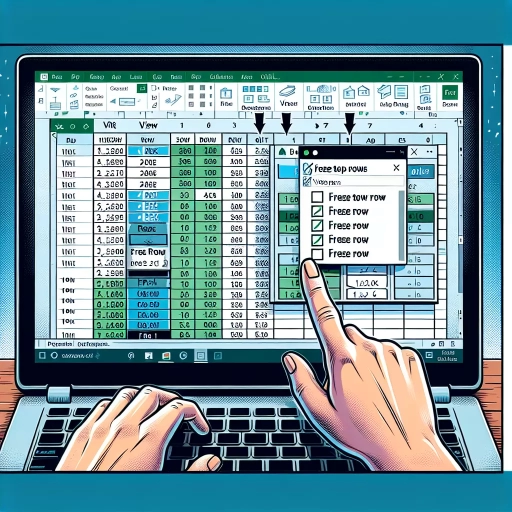
Step 2 of our step-by-step guide involves navigating to the 'View' tab and clicking on 'Freeze Panes'. After you have selected your dataset in Excel, you must direct your attention to the top of the screen where the toolbars are located. Here, you will find diverse tabs like 'Home', 'Insert', 'Page Layout', and more. You need to find and click on the 'View' tab, the one that's usually located towards the far right. The 'View' tab is quite versatile, equipped with numerous benefits that can enhance your efficiency while working with Excel documents. Within the multitude of features that this tab has to offer, there's one particularly crucial function in the context of this guide — 'Freeze Panes'. Upon clicking the 'View' tab, you will see a collection of different icons and titles arranged strategically. Find and click on 'Freeze Panes', usually located in the 'Window' grouping of commands. This icon illustrates a small window, further split into two sections, seemingly 'frozen' in place. Your cursor should be in the second row of your document, the row you wish to freeze along with the top one. By clicking on 'Freeze Panes', it opens a drop-down menu which further provides three distinctive options; 'Freeze Panes', 'Freeze Top Row', and 'Freeze First Column'. This feature acts like a digital steadfast clip that retains the selected rows or columns in its original place, continuing to display them as you scroll through your document. This technique is especially beneficial when your report extends beyond the visible screen area enabling efficient data tracking and management. This little trick can save you from constant scrolling up and down when dealing with voluminous data sets. Remember, the 'Freeze Panes' option would be ineffective if not used correctly. It's essential to place your cursor in the correct cell ahead of going to the step of selecting the freeze option. Since we aim to freeze the top two rows, the cursor should ideally be in the beginning cell of the third row. Excel freezes the rows above and the columns to the left of the selected cell, thus this step is necessary for successful implementation. As you implement this, you will notice the selected rows remain visually static while others scroll, ensuring you are never out of context with your comprehensive data set. The concept of freezing panes has truly revolutionized the approach to data navigation, favoring a more user-friendly, efficient, and robust mechanism for competent and easy data management in Excel.

Step 3: Choose the Freeze Panes Option

Considering the essential role that proper data visibility plays in producing accurate and comprehensive outcomes, the process of freezing the top two rows in Excel becomes a necessary skill to acquire. Now that you have prepared your data and navigated onto the tab that displays 'view options,' we transition onto to step 3, which expands on choosing the 'Freeze Panes' feature. This feature is specifically designed to increase the functionality of your Excel worksheet, particularly when dealing with an extensive database. The 'Freeze Panes' option can be found in the 'Window' group of the 'View' tab in the Excel toolbar. This function, as suggested by its name, freezes, locks or immobilizes a specific portion of the worksheet, primarily columns or rows, while the rest remain active for scrolling. This allows users to continue viewing critical data in the frozen section as they navigate throughout the worksheet, which especially comes in handy when dealing with large datasheets. This simultaneous viewing grants the ability to compare and analyze data more effectively, enhancing productivity and reducing errors due to the misuse of data. Choosing 'Freeze Panes' does not require too much detail or confusion - merely clicking the option opens up a drop-down list with three more options: 'Freeze Panes,' 'Freeze Top Row,' and 'Freeze First Column.' If you need the first two rows to remain visible at all times while scrolling, choose the 'Freeze Panes' option, ensuring you have clicked on the cell in the third row before doing so. This selection has now converted your standard worksheet into a vast, easily maneuverable database with organized, viewable sections to optimize data analysis. In conclusion, Excel's 'Freeze Panes' is a vital, practical function for users to increase the convenience and efficiency of navigating through large data sets. It is a tool that can be easily accessed and operated, eliminating the need for constant scrolling and reducing the associated risk of human error in data handling. The selection of the 'Freeze Panes' option marks a significant step towards maintaining clarity within your Excel worksheet infrastructure, catering to data requirements, and delivering a reproducible system of organization.

Customizing and Managing Frozen Rows in Excel

of any data analysis or presentation is the effective use of Excel, a powerful tool with diverse features. One such feature, often overlooked for its seeming simplicity but incredibly essential, is the 'Freeze Rows' function. This feature provides a more optimized view of data by keeping certain rows or columns visible while you scroll through your data sheet. To enhance your proficiency in excel, this article would elucidate how to customize and manage frozen rows, accentuating three key areas: "Freezing Multiple Rows in Excel," "Unfreezing Frozen Rows in Excel," and "Freezing Rows in Excel with Formulas and Functions." Firstly, we will get into the nitty-gritty of managing multiple rows in one freeze pane. This handy trick can help you keep track of multiple headers while navigating through extensive data on excel sheets. Thus, enabling you to customize view management, which not only amplifies your productivity but also conserves significant amounts of time. So, without any further ado, let's delve into our first topic: "Freezing Multiple Rows in Excel."

Freezing Multiple Rows in Excel

Freezing multiple rows in Excel is a vital feature that improves the overall experience and effectiveness while handling sizable data. This feature provides a seamless way for users to keep track of important data in rows or columns while scrolling through other parts of the worksheet. By freezing rows, there's absolutely no need to repeatedly scroll up to remind oneself about the data extrapolations or headings, as those will always be visible. Freezing multiple rows can apply to various fields such as financial analysis, research work, data entry, project planning, etc. Imagine dealing with a spreadsheet that populates product sales data, where column headings bear details like product names, customer details, sales figures, etc. Navigating through extensive data sheets without losing sight of these column headings can turn into quite a daunting task without the 'freeze panes' option. Moreover, this feature is extremely user-friendly and accessible, even to beginners. Excel allows freezing from one to multiple rows based on user preference. To freeze multiple rows, select the row below the last one you wish to freeze, navigate to the 'View' tab, choose the 'Freeze Panes' drop-down option, and click 'Freeze Panes.' Voila, your rows are frozen, and it's as simple as that! You can scroll down, and the frozen rows will remain visible at the top of Excel, aiding you in managing your data effectively. Furthermore, Excel offers customizable features in managing these frozen rows. For instance, users can 'unfreeze' rows whenever they want to revert the sheet to its original state. Also, users have the liberty to freeze both rows and columns simultaneously. By specifically pinpointing the cell where the rows and columns intersect and selecting the 'Freeze Panes' option again, users can manage their data more efficiently. For instance, while managing monthly sales data, users may want to freeze the top row representing each month and the first column representing each product, enabling a smoother navigation through the data, irrespective of its volume and complexity. Overall, Excel's feature to freeze multiple rows maximizes productivity by minimizing the potential for errors and confusion that comes with handling large datasets. Whether you're an analyst crunching numbers, a researcher analyzing data, or a student working on a project, the ability to freeze and manage multiple rows in Excel, coupled with the potential for customization, can significantly elevate your data handling and interpreting capabilities. Always remember, effective data management is key to precision in data interpretation, making the freeze feature an indispensable tool in the world of spreadsheets.

Unfreezing Frozen Rows in Excel

When handling large datasets in Excel, freezing rows is a beneficial feature that enhances the accessibility of vital data. Despite the numerous benefits, there may come a time when it becomes essential to unfreeze these rows for various reasons such as to edit or modify data, customize the view, or manage the worksheet's layout more effectively. Unfreezing rows in Excel is a quick and straightforward process. You begin by selecting the 'View' tab on the Excel ribbon, which is the third tab from the right on the Excel Home Screen. After clicking on 'View,' a drop-down menu appears, and you have to select 'Freeze Panes.' Upon selecting 'Freeze Panes,' another submenu will open, and you’ll see the 'Unfreeze Panes' option. By clicking on 'Unfreeze Panes,' any previously frozen rows or columns in your worksheet will be unfrozen immediately. This procedure applies to all versions of Excel, and it allows users to effortlessly navigate the worksheet. The feature to unfreeze panes comes in handy when you need to customize or change the frozen rows. For instance, you may want to freeze or unfreeze different rows based on the task at hand. It also proves useful when extensive editing or formatting comes into the picture; it provides the flexibility users need when managing complex spreadsheets. Understanding how to unfreeze rows is therefore crucial for efficient and effective data management in Excel. However, it is imperative to remember the process of unfreezing rows doesn't automatically revert to the original state before the rows were frozen. Once the rows are unfrozen, you will need to manually scroll to find the desired data. This factor is worth considering, especially when working with large datasets—specifically, if the data you are frequently accessing had been in the now unfrozen rows. A pro tip while dealing with this Excel feature is, before unfreezing rows, always remember to note down which rows were frozen initially. This way, if you want to revert, you won't miss out on freezing any critical data row. It's a small but proactive step that can save you a considerable amount of trouble in case you quickly need to freeze the same row again. Thus, while the ability to freeze panes in Excel considerably improves the user's navigating experience, the flexibility to unfreeze frozen rows when required makes Excel a dynamic tool for handling and presenting data efficiently.

Freezing Rows in Excel with Formulas and Functions

Excel, being an analytics powerhouse, offers numerous ways for customizing rows and columns. Indeed, one of the most beneficial feature for precision formatting and organization is the ability to freeze rows. When dealing with extensive data sets, it becomes increasingly challenging to manage the data effectively. However, with freezing rows in Excel, along with Formulas and Functions, you can lock rows while scrolling, ensuring that specific data is constantly visible. For instance, imagine working with a data set where the first two rows include the most important information such as the column labels or key figures. Evidently, when you scroll down, you'd want these rows to always be visible for a point of reference. Here's where Excel’s freeze rows feature comes into play. By selecting 'Freeze Panes' from the 'View' tab, you can easily lock in the top two rows no matter how far down you scroll. In this way, Excel’s freezing functionality not only amplifies your user experience by negating the need to memorize or continuously revert to top, but it also enhances the accuracy of your data management. Yet, freezing rows become even more powerful when combined with Excel’s Formulas and Functions. You can apply formulas and functions in frozen rows to perform calculations, like sum or average, which then persist as you scroll through the data. This consistency of calculations is immensely beneficial for tasks such as financial analysis, where totals, averages and trends of large data sets need to be evaluated frequently. By customizing the formulas for frozen rows, you can establish a dynamic table where calculations in the locked rows automatically adjust depending on the data in the unfrozen section of the spreadsheet. This sophisticated setup allows you to make live updates, both swiftly and accurately. For example, imagine having a monthly sales report with a total revenue calculation in a frozen row. As you input the daily sales throughout the month in the scrollable rows below, the frozen total revenue cell would instantly reflect the new sum. In conclusion, the integration of freezing rows in Excel with Formulas and Functions brings about an enormous gain in terms of efficiency, precision, and overall data management. Delving more into customizing and managing frozen rows, you can further explore Excel's vast functionalities and obtain valuable insights from your data quicker and with much less effort. In the realm of digital data analysis, something as simple as freezing rows can significantly streamline operations - a testament to Excel's potential in enhancing productivity.