Here is the introduction paragraph: When working with charts and graphs in Excel, it's essential to have a clear and concise way to identify and differentiate between various data series. One way to achieve this is by assigning meaningful names to each series, making it easier to understand and analyze the data. However, changing the series name in Excel can be a bit tricky, especially for those who are new to the software. In this article, we will explore the basics of series names in Excel, discuss various methods to change series names, and provide advanced techniques for managing series names. By the end of this article, you will be able to confidently change series names in Excel and take your data analysis to the next level. To get started, let's first understand the basics of series names in Excel.

Understanding the Basics of Series Names in Excel

When working with data in Excel, creating informative and engaging charts is crucial for effective communication and analysis. One often overlooked aspect of chart creation is the series name, which plays a vital role in conveying the meaning and context of the data. Understanding the basics of series names in Excel is essential for creating high-quality charts that accurately represent the data. In this article, we will explore the importance of series names in Excel charts, how they behave by default, and what they are. By grasping these fundamental concepts, users can unlock the full potential of their charts and make more informed decisions. So, let's start by understanding what series names are in Excel.

What are Series Names in Excel?

In Excel, a series name is a label that identifies a specific set of data points in a chart. It is used to differentiate one set of data from another, especially when multiple series are plotted on the same chart. Series names are typically displayed in the legend of the chart, making it easier to understand and interpret the data. By default, Excel assigns a generic name to each series, such as "Series 1," "Series 2," and so on. However, you can customize these names to make them more descriptive and meaningful. For example, if you have a chart that shows sales data for different regions, you can rename the series to "North," "South," "East," and "West" to make it clearer which series represents which region. Customizing series names can greatly enhance the readability and effectiveness of your charts, making it easier for your audience to understand the data and insights you are trying to convey.

Why are Series Names Important in Excel Charts?

When it comes to creating effective and informative charts in Excel, series names play a crucial role. Series names are the labels that identify each data series in a chart, and they are essential for several reasons. Firstly, series names help to clarify the data being presented, making it easier for viewers to understand the chart and its components. Without clear series names, a chart can be confusing and difficult to interpret, leading to miscommunication and incorrect conclusions. Secondly, series names enable users to customize the appearance of their charts, allowing them to choose colors, fonts, and other formatting options that best represent their data. This level of customization is particularly important in professional settings, where charts are often used to present complex data to clients, stakeholders, or colleagues. Furthermore, series names are also important for data analysis and comparison. By clearly labeling each data series, users can easily compare and contrast different data sets, identify trends and patterns, and make informed decisions. In addition, series names can also be used to create dynamic charts that update automatically when new data is added or changed. Overall, series names are a critical component of effective chart creation in Excel, and understanding how to use them is essential for anyone looking to create informative and engaging charts.

Default Series Name Behavior in Excel

When creating a chart in Excel, the default series name behavior can be a bit confusing, especially for those new to charting. By default, Excel assigns a series name based on the header cell of the data range used to create the chart. This means that if your data range has a header row, Excel will use the text in the header cell as the series name. However, if your data range does not have a header row, Excel will assign a default series name, such as "Series 1," "Series 2," and so on. This default behavior can lead to charts with unclear or misleading series names, making it difficult to interpret the data. To avoid this, it's essential to understand how to change the series name in Excel, which can be done by editing the series name in the chart's data source or by using the "Select Data" feature in the chart's design tab. By taking control of the series name, you can ensure that your charts are clear, concise, and easy to understand, making it easier to communicate insights and trends to your audience.

Methods to Change Series Name in Excel

Here is the introduction paragraph: Changing the series name in Excel can be a bit tricky, but there are several methods to achieve this. In this article, we will explore three effective methods to change the series name in Excel. The first method involves changing the series name through the chart source data, which is a straightforward approach. The second method involves using the formula bar to change the series name, which is useful when working with complex formulas. The third method involves using the select data source dialog box, which provides more flexibility in changing the series name. In this article, we will delve into each of these methods in detail, starting with the first method: changing series name through the chart source data.

Method 1: Changing Series Name through the Chart Source Data

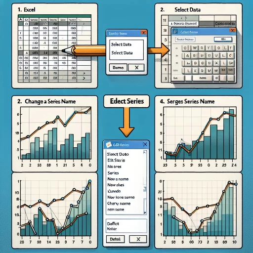
To change the series name in Excel through the chart source data, follow these steps. First, select the chart for which you want to change the series name. Then, click on the "Chart Design" tab in the ribbon. In the "Data" group, click on the "Select Data" button. This will open the "Select Data Source" dialog box. In this dialog box, you will see a list of all the series in your chart. Click on the series for which you want to change the name, and then click on the "Edit" button. In the "Edit Series" dialog box, you can change the series name in the "Series name" field. You can also change the series formula and the range of cells that the series is based on. Once you have made the changes, click on the "OK" button to close the dialog box. The series name will be updated in the chart. This method is useful when you want to change the series name for a specific chart, and you don't want to change the underlying data.

Method 2: Changing Series Name through the Formula Bar

To change the series name in Excel through the formula bar, follow these steps. First, select the chart that contains the series you want to rename. Then, click on the series to select it. Next, go to the formula bar, which is located at the top of the Excel window, and click on the name of the series. The name will be highlighted, and you can start typing the new name. As you type, the name will be updated in real-time. Once you have entered the new name, press Enter to apply the changes. The series name will be updated in the chart, and the new name will be reflected in the legend and other chart elements. This method is quick and easy, and it allows you to change the series name without having to access the chart's properties or settings. Additionally, you can use this method to change the series name for multiple series at once by selecting all the series you want to rename and then typing the new name in the formula bar.

Method 3: Changing Series Name through the Select Data Source Dialog Box

To change the series name in Excel through the Select Data Source dialog box, follow these steps. First, click on the chart for which you want to change the series name. Then, navigate to the "Chart Design" tab in the ribbon. Click on the "Select Data" button in the "Data" group. This will open the "Select Data Source" dialog box. In this dialog box, you will see a list of all the series in your chart. Click on the series for which you want to change the name. Then, click on the "Edit" button. In the "Edit Series" dialog box, you will see a field labeled "Series name." Type the new name for the series in this field. Click "OK" to apply the changes. The series name will be updated in the chart. This method is useful when you want to change the series name for a specific chart, and you don't want to change the data source. By using the Select Data Source dialog box, you can easily change the series name without affecting the underlying data.

Advanced Techniques for Managing Series Names in Excel

When working with large datasets in Excel, managing series names can be a daunting task. However, with the right techniques, you can streamline your workflow and make your charts and graphs more informative. In this article, we will explore advanced techniques for managing series names in Excel, including using dynamic series names with formulas, renaming multiple series names at once, and best practices for series name management. By mastering these techniques, you can take your Excel skills to the next level and create more effective and engaging visualizations. One of the most powerful techniques for managing series names is using dynamic series names with formulas, which allows you to automatically update your series names based on changes to your data. By using formulas to define your series names, you can ensure that your charts and graphs always reflect the latest information, without having to manually update the series names. In the next section, we will dive deeper into using dynamic series names with formulas and explore how to implement this technique in your own Excel spreadsheets.

Using Dynamic Series Names with Formulas

Using dynamic series names with formulas is a powerful technique in Excel that allows you to automatically update your chart series names based on changes in your data. This approach eliminates the need for manual updates and ensures that your chart remains accurate and up-to-date. To implement dynamic series names with formulas, you can use a combination of Excel functions such as OFFSET, INDEX, and MATCH. For instance, you can use the OFFSET function to reference a cell range that contains the series names, and then use the INDEX and MATCH functions to dynamically retrieve the correct series name based on the data. Another approach is to use a named range or a table to store the series names, and then use a formula to reference the named range or table. By using dynamic series names with formulas, you can create flexible and dynamic charts that automatically adjust to changes in your data, making it easier to analyze and visualize your data. Additionally, this technique can be used in conjunction with other advanced techniques, such as using multiple series in a single chart, to create complex and informative charts. Overall, using dynamic series names with formulas is a valuable skill for any Excel user looking to take their charting and data analysis skills to the next level.

Renaming Multiple Series Names at Once

Renaming multiple series names at once in Excel can be a significant time-saver, especially when dealing with large datasets or multiple charts. To achieve this, you can use the "Select Data" feature in the chart tools. Start by clicking on the chart that contains the series you want to rename. Then, navigate to the "Chart Tools" section in the ribbon and click on "Select Data." In the "Select Data Source" dialog box, you'll see a list of all the series in your chart. To rename multiple series at once, hold down the "Ctrl" key and select the series you want to rename. Once you've selected the series, click on the "Edit" button and enter the new name for the series. You can also use the "Rename" feature in the "Series" section of the "Chart Tools" to rename multiple series at once. Another approach is to use VBA macros to rename multiple series names at once. This method requires some programming knowledge, but it can be a powerful tool for automating repetitive tasks. By using VBA macros, you can write a script that loops through all the series in your chart and renames them according to your specifications. This can be especially useful if you need to rename series names in multiple charts or worksheets. Overall, renaming multiple series names at once in Excel can be a convenient and efficient way to manage your data and improve the readability of your charts.

Best Practices for Series Name Management in Excel

When managing series names in Excel, it's essential to follow best practices to ensure accuracy, consistency, and ease of use. One of the most critical best practices is to use a standardized naming convention for series names. This involves using a consistent format, such as "Category - Subcategory" or "Region - Product," to make it easy to identify and distinguish between different series. Another best practice is to avoid using special characters, such as asterisks or slashes, in series names, as they can cause issues with formulas and charts. Additionally, it's recommended to keep series names concise and descriptive, avoiding unnecessary words or characters. This not only makes it easier to read and understand the data but also helps to prevent errors when working with formulas and charts. Furthermore, it's a good idea to use a separate column or table to store series names, rather than hardcoding them into formulas or charts. This allows for easy maintenance and updates, as well as the ability to reuse series names across multiple charts and reports. By following these best practices, users can ensure that their series names are accurate, consistent, and easy to manage, making it easier to create effective and informative charts and reports in Excel.