When creating charts in Excel, axis labels play a crucial role in making the data more readable and understandable. However, many users struggle with adding and customizing these labels, which can lead to confusion and misinterpretation of the data. In this article, we will explore the world of axis labels in Excel, starting with the basics of what they are and how they work. We will then dive into the practical steps of adding axis labels to your charts, including tips and tricks for customizing their appearance and behavior. Finally, we will take it to the next level by exploring advanced techniques for customizing axis labels, such as using formulas and formatting options. By the end of this article, you will be equipped with the knowledge and skills to create professional-looking charts with clear and effective axis labels. So, let's start by understanding the basics of axis labels in Excel.

Understanding the Basics of Axis Labels in Excel

When creating charts in Excel, it's essential to understand the basics of axis labels to effectively communicate your data insights. Axis labels are a crucial component of any chart, as they provide context and meaning to the data being presented. In this article, we'll delve into the world of axis labels, exploring what they are, the different types available in Excel, and the benefits of using them in your charts. By the end of this article, you'll have a solid understanding of how to use axis labels to enhance your data visualization and make your charts more informative and engaging. So, let's start by understanding the fundamentals of axis labels and why they're so important in Excel charts. What are Axis Labels and Why are They Important?

What are Axis Labels and Why are They Important?

Axis labels are the text or numbers that appear along the x-axis and y-axis of a chart in Excel, providing context and meaning to the data being displayed. They are essential components of a chart, as they help viewers understand the data points and trends being represented. Axis labels can include titles, such as "Sales" or "Revenue," as well as numerical values, like "0" to "100." By including axis labels, you can ensure that your chart is clear, concise, and easy to interpret, making it more effective at communicating insights and trends to your audience. Furthermore, axis labels can also help to prevent misinterpretation of data, as they provide a clear frame of reference for the data points being plotted. In Excel, you can customize axis labels to suit your needs, choosing from a range of options, including font styles, colors, and sizes. By taking the time to add and customize axis labels, you can create charts that are not only visually appealing but also informative and effective at conveying your message.

Types of Axis Labels in Excel

In Excel, axis labels are a crucial component of charts, providing context and clarity to the data being presented. There are several types of axis labels that can be used in Excel, each serving a specific purpose. The most common types of axis labels are numerical labels, which display numerical values along the axis. These labels can be customized to display specific number formats, such as currency or percentage. Another type of axis label is the categorical label, which displays text labels for each category or group in the data. These labels can be used to identify specific groups or categories in the data, making it easier to compare and analyze. Date and time labels are also commonly used in Excel, particularly when working with time-series data. These labels display dates and times along the axis, allowing users to easily identify trends and patterns in the data. Additionally, Excel also supports the use of custom labels, which can be created using formulas or text strings. These labels can be used to add additional context or information to the chart, such as labels for specific data points or annotations. Overall, the type of axis label used in Excel will depend on the specific needs of the chart and the data being presented.

Benefits of Using Axis Labels in Excel Charts

Using axis labels in Excel charts can greatly enhance the readability and effectiveness of your visualizations. By adding labels to your axes, you can provide context and clarity to your data, making it easier for your audience to understand the information being presented. One of the primary benefits of using axis labels is that they help to avoid confusion and misinterpretation of the data. Without labels, viewers may struggle to comprehend the meaning of the data points, leading to incorrect conclusions. By clearly labeling the axes, you can ensure that your audience accurately interprets the data and draws the intended insights. Additionally, axis labels can also help to highlight trends and patterns in the data, making it easier to identify key takeaways and insights. Furthermore, using axis labels can also improve the overall aesthetic of your chart, making it more visually appealing and professional. By incorporating labels into your axes, you can create a more polished and sophisticated visualization that effectively communicates your message. Overall, the benefits of using axis labels in Excel charts are numerous, and by incorporating them into your visualizations, you can create more effective, informative, and engaging charts that accurately convey your data insights.

Adding Axis Labels to Your Excel Charts

When creating charts in Excel, adding axis labels is a crucial step to ensure that your data is presented in a clear and understandable manner. Axis labels provide context to the data being displayed, making it easier for viewers to comprehend the information. In this article, we will explore three methods for adding axis labels to your Excel charts. First, we will discuss how to use the Chart Elements button to add axis labels, a quick and easy method that can be done with just a few clicks. Additionally, we will cover how to manually add axis labels through the Format Axis option, which provides more customization options. Finally, we will touch on how to customize axis labels for better readability, including tips on font size, color, and alignment. By the end of this article, you will be equipped with the knowledge to effectively add axis labels to your Excel charts, starting with the simplest method: using the Chart Elements button to add axis labels.

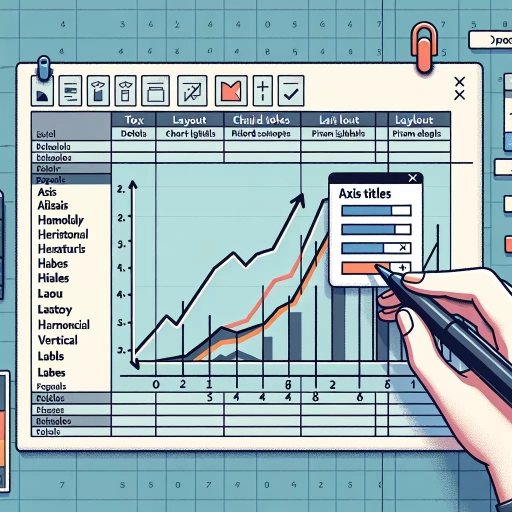
Using the Chart Elements Button to Add Axis Labels

To add axis labels to your Excel charts, you can use the Chart Elements button, which provides a quick and easy way to customize your chart's appearance. The Chart Elements button is located in the upper-right corner of your chart and is represented by a plus sign (+). When you click on this button, a menu will appear with various options for adding different elements to your chart, including axis labels. To add axis labels, simply click on the "Axis Titles" option from the menu, and then select the type of axis label you want to add, such as "Primary Horizontal" or "Primary Vertical". You can also customize the appearance of your axis labels by clicking on the "More Options" button, which will open the "Format Axis Title" pane. From here, you can change the font, color, and alignment of your axis labels, as well as add a title to your axis. Additionally, you can use the "Chart Elements" button to add other elements to your chart, such as a chart title, legend, or data labels, allowing you to fully customize your chart to meet your needs. By using the Chart Elements button, you can easily add axis labels to your Excel charts and enhance their overall appearance and effectiveness.

Manually Adding Axis Labels through the Format Axis Option

When manually adding axis labels through the Format Axis option, you have complete control over the appearance and placement of the labels. To access this feature, select the axis for which you want to add labels, go to the "Format" tab in the ribbon, and click on "Format Axis." In the Format Axis pane, click on the "Labels" option, and then select "Specify Interval Unit" to set the interval at which the labels appear. You can also choose to display labels at specific positions, such as at the minimum, maximum, or midpoint of the axis. Additionally, you can customize the label's font, size, color, and alignment to match your chart's style. Furthermore, you can add a title to the axis by checking the "Axis title" box and typing in the desired text. This feature allows you to add context to your chart and make it easier to understand. By manually adding axis labels through the Format Axis option, you can enhance the readability and visual appeal of your Excel charts.

Customizing Axis Labels for Better Readability

Customizing axis labels is a crucial step in enhancing the readability of your Excel charts. By default, Excel generates axis labels based on the data in your chart, but these labels may not always be clear or concise. To improve the readability of your chart, you can customize the axis labels to better suit your needs. One way to do this is by changing the font size, style, and color of the labels. You can also adjust the label alignment and orientation to make them easier to read. Additionally, you can add prefixes or suffixes to the labels to provide more context, such as adding a currency symbol or a unit of measurement. Furthermore, you can use the "Number" section in the "Format Axis" dialog box to specify the number of decimal places or the date format for the labels. By customizing the axis labels, you can make your chart more informative and easier to understand, which is especially important when presenting data to others.

Advanced Techniques for Customizing Axis Labels

When it comes to customizing axis labels in charts, there are several advanced techniques that can elevate the visualization and communication of data insights. One of the key challenges in data visualization is effectively conveying complex information in a clear and concise manner. By leveraging advanced techniques for customizing axis labels, users can create more informative and engaging charts that facilitate better decision-making. Three essential techniques for achieving this include using formulas to create dynamic axis labels, adding multiple axis labels to a single chart, and rotating and formatting axis labels for enhanced visualization. By mastering these techniques, users can unlock new possibilities for data storytelling and presentation. For instance, using formulas to create dynamic axis labels can help automate the process of updating labels, ensuring that charts remain accurate and up-to-date. This technique is particularly useful for charts that require frequent updates, such as those used in real-time data monitoring or reporting. By using formulas to create dynamic axis labels, users can streamline their workflow and focus on higher-level analysis and insights.

Using Formulas to Create Dynamic Axis Labels

Using formulas to create dynamic axis labels is a powerful technique in Excel that allows you to automatically update your axis labels based on changes in your data. This approach is particularly useful when working with dynamic data that frequently changes, such as sales figures or stock prices. To create dynamic axis labels using formulas, start by selecting the cell that contains the data you want to use as the label. Then, go to the "Formula" tab in the ribbon and click on the "Define Name" button. In the "New Name" dialog box, give your formula a name, such as "AxisLabel," and enter the formula that will generate the label text. For example, if you want to display the current month as the axis label, you can use the formula "=TEXT(TODAY(),"MMMM")". Once you've defined the formula, go back to the chart and select the axis label you want to update. Right-click on the label and select "Format Axis Label." In the "Format Axis Label" dialog box, click on the "Formula" button and select the formula you defined earlier. Click "OK" to apply the changes. Now, whenever you update your data, the axis label will automatically update to reflect the new values. You can also use formulas to create more complex axis labels, such as labels that display multiple values or labels that use conditional formatting. For example, you can use the formula "=IF(A1>10,"High","Low")" to create a label that displays "High" if the value in cell A1 is greater than 10, and "Low" otherwise. By using formulas to create dynamic axis labels, you can add an extra layer of sophistication to your charts and make them more interactive and engaging.

Adding Multiple Axis Labels to a Single Chart

When working with complex data visualizations in Excel, it's not uncommon to need multiple axis labels on a single chart. This can be particularly useful when dealing with multiple data series that have different units or scales. Fortunately, Excel provides a few different methods for adding multiple axis labels to a single chart. One approach is to use the "Secondary Axis" feature, which allows you to add a second axis to your chart and customize its labels independently of the primary axis. To do this, select the data series you want to display on the secondary axis, go to the "Chart Tools" tab, and click on the "Axes" button. From there, you can choose to add a secondary axis and customize its labels as needed. Another approach is to use the "Axis Title" feature, which allows you to add a title to your axis and customize its text and formatting. To do this, select the axis you want to add a title to, go to the "Chart Tools" tab, and click on the "Axis Title" button. From there, you can enter the text you want to display as the axis title and customize its formatting as needed. You can also use a combination of both methods to add multiple axis labels to a single chart. For example, you can add a secondary axis and then add an axis title to each axis to provide additional context and clarity. By using these techniques, you can create complex and informative charts that effectively communicate your data insights to your audience.

Rotating and Formatting Axis Labels for Enhanced Visualization

When it comes to creating effective and informative charts in Excel, rotating and formatting axis labels can make a significant difference in enhancing visualization. By default, Excel displays axis labels horizontally, but this can sometimes lead to overlapping or cramped labels, making it difficult to read and understand the data. Rotating axis labels can help to alleviate this issue and improve the overall appearance of the chart. To rotate axis labels, simply select the axis label range, go to the "Home" tab, and click on the "Orientation" button in the "Alignment" group. From here, you can choose from a variety of rotation options, including 90 degrees, 45 degrees, and more. Additionally, you can also use the "Text Direction" button to change the direction of the text from horizontal to vertical or vice versa. Formatting axis labels is also crucial in enhancing visualization. You can change the font, size, color, and style of the labels to match your chart's theme and make them more readable. For example, you can use a larger font size for the x-axis labels and a smaller font size for the y-axis labels to create a clear visual hierarchy. You can also use bold or italic text to draw attention to specific labels or use different colors to differentiate between different categories. Furthermore, you can also add borders, shadows, or other effects to the labels to make them stand out. By rotating and formatting axis labels, you can create a more visually appealing and effective chart that communicates your data insights more clearly. This, in turn, can help to engage your audience, facilitate better decision-making, and ultimately drive business success.